models
|
a model, (named) list of models, or nested list of models.
-
Single model: modelsummary(model)
-
Unnamed list of models: modelsummary(list(model1, model2))
-
Named list of models: modelsummary(list(“A”=model1, “B”=model2))
-
Nested list of models:
-
When using the shape argument with "rbind", "rcollapse", or "cbind" values, models can be a nested list of models to display "panels" or "stacks" of regression models. See the shape argument documentation and examples below.
|
conf_level
|
numeric value between 0 and 1. confidence level to use for confidence intervals. Setting this argument to NULL does not extract confidence intervals, which can be faster for some models.
|
coef_map
|
character vector. Subset, rename, and reorder coefficients. Coefficients omitted from this vector are omitted from the table. The order of the vector determines the order of the table. coef_map can be a named or an unnamed character vector. If coef_map is a named vector, its values define the labels that must appear in the table, and its names identify the original term names stored in the model object: c(“hp:mpg”=“HPxM/G”). If coef_map is an unnamed vector, its values must be raw variable names if coef_rename=FALSE and variable labels if coef_rename=TRUE. See modelsummary::get_estimates to get the coefficient out of a model. See Examples section below.
|
coef_omit
|
integer vector or regular expression to identify which coefficients to omit (or keep) from the table. Positive integers determine which coefficients to omit. Negative integers determine which coefficients to keep. A regular expression can be used to omit coefficients, and perl-compatible "negative lookaheads" can be used to specify which coefficients to keep in the table. Examples:
-
c(2, 3, 5): omits the second, third, and fifth coefficients.
-
c(-2, -3, -5): negative values keep the second, third, and fifth coefficients.
-
“ei”: omit coefficients matching the "ei" substring.
-
“^Volume$”: omit the "Volume" coefficient.
-
“ei|rc”: omit coefficients matching either the "ei" or the "rc" substrings.
-
“^(?!Vol)”: keep coefficients starting with "Vol" (inverse match using a negative lookahead).
-
“^(?!.*ei)“: keep coefficients matching the”ei" substring.
-
“^(?!.ei|.pt)”: keep coefficients matching either the "ei" or the "pt" substrings.
-
See the Examples section below for complete code.
|
coef_rename
|
logical, named or unnamed character vector, or function
-
Logical: TRUE renames variables based on the "label" attribute of each column. See the Example section below. Note: renaming is done by the parameters package at the extraction stage, before other arguments are applied like coef_omit. Therefore, this only works for models with builtin support and not for custom models.
-
Unnamed character vector of length equal to the number of coefficients in the final table, after coef_omit is applied.
-
Named character vector: Values refer to the variable names that will appear in the table. Names refer to the original term names stored in the model object. Ex: c("hp:mpg"="hp X mpg")
-
Function: Accepts a character vector of the model’s term names and returns a named vector like the one described above. The modelsummary package supplies a coef_rename() function which can do common cleaning tasks: modelsummary(model, coef_rename = coef_rename)
|
vcov
|
robust standard errors and other manual statistics. The vcov argument accepts six types of input (see the ‘Details’ and ‘Examples’ sections below):
-
NULL returns the default uncertainty estimates of the model object
-
string, vector, or (named) list of strings. "iid", "classical", and "constant" are aliases for NULL, which returns the model’s default uncertainty estimates. The strings "HC", "HC0", "HC1" (alias: "stata"), "HC2", "HC3" (alias: "robust"), "HC4", "HC4m", "HC5", "HAC", "NeweyWest", "Andrews", "panel-corrected", "outer-product", and "weave" use variance-covariance matrices computed using functions from the sandwich package, or equivalent method. "BS", "bootstrap", "residual", "mammen", "webb", "xy", "wild" use the sandwich::vcovBS(). The behavior of those functions can (and sometimes must) be altered by passing arguments to sandwich directly from modelsummary through the ellipsis (…), but it is safer to define your own custom functions as described in the next bullet.
-
function or (named) list of functions which return variance-covariance matrices with row and column names equal to the names of your coefficient estimates (e.g., stats::vcov, sandwich::vcovHC, function(x) vcovPC(x, cluster=“country”)).
-
formula or (named) list of formulas with the cluster variable(s) on the right-hand side (e.g., ~clusterid).
-
named list of length(models) variance-covariance matrices with row and column names equal to the names of your coefficient estimates.
-
a named list of length(models) vectors with names equal to the names of your coefficient estimates. See ‘Examples’ section below. Warning: since this list of vectors can include arbitrary strings or numbers, modelsummary cannot automatically calculate p values. The stars argument may thus use incorrect significance thresholds when vcov is a list of vectors.
|
exponentiate
|
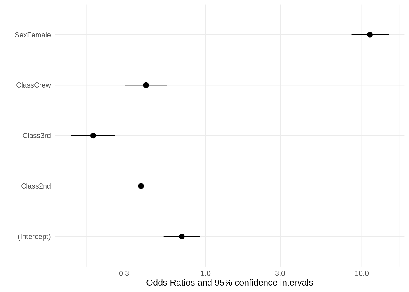
TRUE, FALSE, or logical vector of length equal to the number of models. If TRUE, the estimate, conf.low, and conf.high statistics are exponentiated, and the std.error is transformed to exp(estimate)*std.error. The exponentiate argument is ignored for distributional random effects parameters (SD and Cor) and dispersions parameters.
|
add_rows
|
a data.frame (or tibble) with the same number of columns as your main table. By default, rows are appended to the bottom of the table. Positions can be defined using integers. In the modelsummary() function (only), you can also use string shortcuts: "coef_start", "coef_end", "gof_start", "gof_end"
|
facet
|
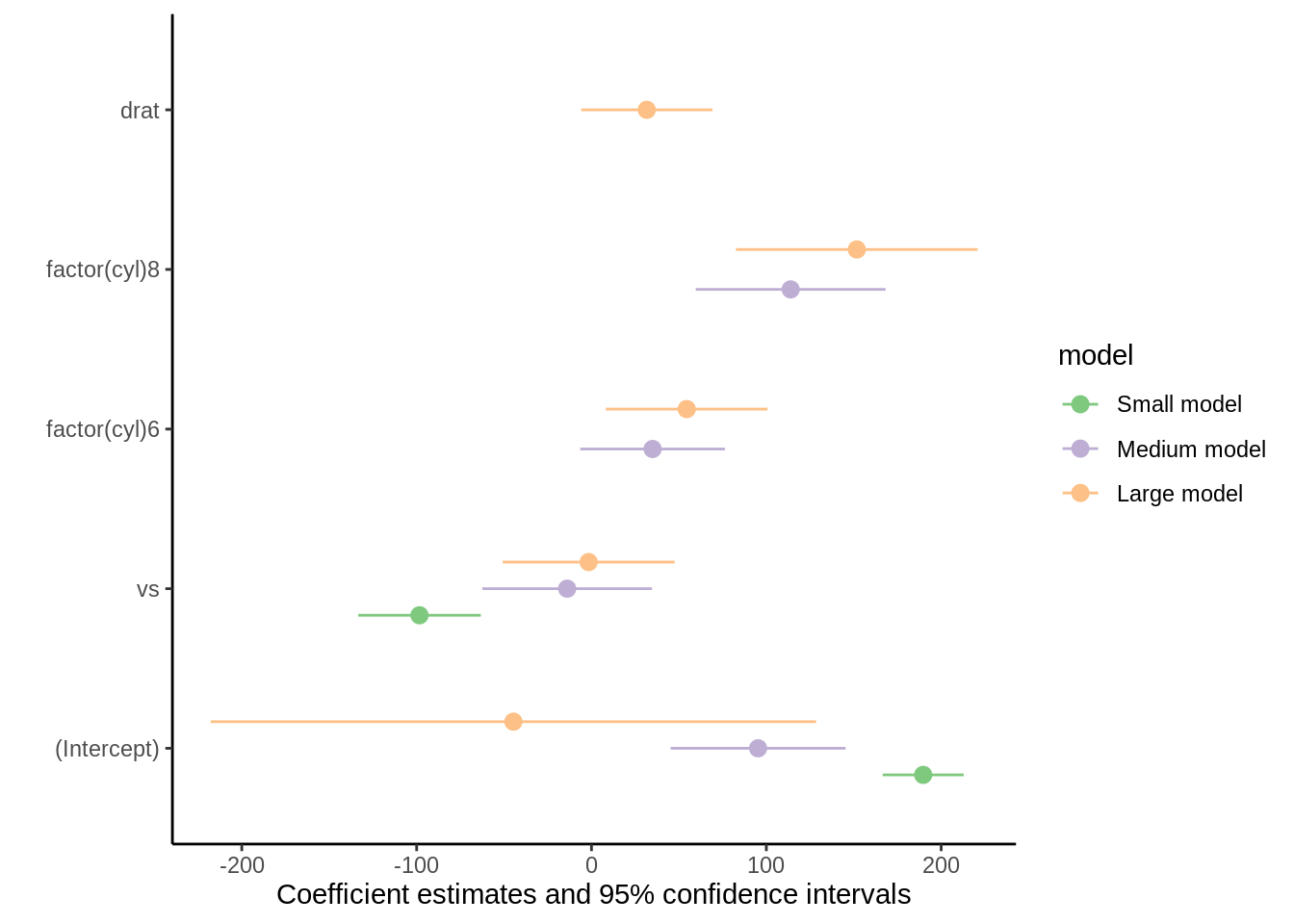
TRUE or FALSE. When the ‘models’ argument includes several model objects, TRUE draws terms in separate facets, and FALSE draws terms side-by-side (dodged).
|
draw
|
TRUE returns a ‘ggplot2’ object, FALSE returns the data.frame used to draw the plot.
|
background
|
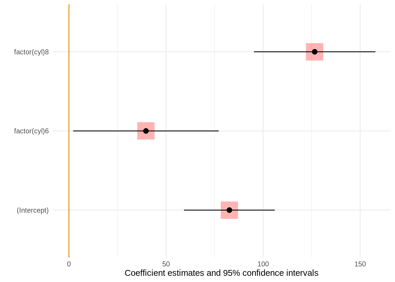
A list of ‘ggplot2’ geoms to add to the background of the plot. This is especially useful to display annotations "behind" the ‘geom_pointrange’ that ‘modelplot’ draws.
|
…
|
all other arguments are passed through to three functions. See the documentation of these functions for lists of available arguments.
-
parameters::model_parameters extracts parameter estimates. Available arguments depend on model type, but include:
-
standardize, include_reference, centrality, dispersion, test, ci_method, prior, diagnostic, rope_range, power, cluster, etc.
-
performance::model_performance extracts goodness-of-fit statistics. Available arguments depend on model type, but include:
-
tinytable::tt, kableExtra::kbl or gt::gt draw tables, depending on the value of the output argument. For example, by default modelsummary creates tables with tinytable::tt, which accepts a width and theme arguments.
|
